Fluid Mechanics

What is a fluid?#

A fluid is a substance that flows and takes the shape of the container it is in. Liquids and gases are both fluids — "fluid" is the broader category, not a synonym for "liquid."

• Liquids are fluids.
• Gases are fluids.

Classification of fluids#

Ideal fluids vs. real (non-ideal) fluids#

• Ideal fluids: inviscid (zero viscosity), incompressible — a hypothetical simplification; no fluid is actually ideal.
• Real (non-ideal) fluids: viscous — this is the defining property, not compressibility. Compressibility varies independently: most liquids are real but still treated as incompressible, while gases are real and compressible.

Newtonian vs. non-Newtonian fluids#

Another way to classify fluids, based on their flow behavior.

Rheology#

Rheology is the study of the flow of a fluid.

A fluid is a substance that undergoes deformation when subjected to shearing stress.

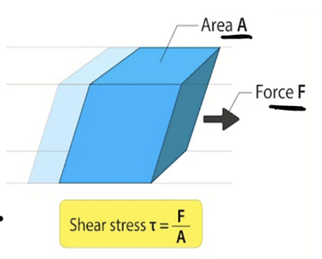
Shear stress#

Shear stress is the tangential force applied per unit area.

$$\tau = \frac{F}{A}$$

• $\tau$ — shear stress (tangential force per unit area, resisting relative sliding between adjacent fluid layers), in pascals ($\text{Pa}$) or newtons per square metre ($\text{N/m}^2$)
• $F$ — tangential force, in newtons ($\text{N}$)
• $A$ — area, in square metres ($\text{m}^2$)

Shear rate#

Shear rate is the strain that occurs within a fluid, representing the change in velocity of adjacent fluid layers over a distance.

A fluid can be thought of as stacked layers, each moving at a different velocity. The topmost layer has no force acting on it from above, so it moves freely. Each layer below experiences a force from the layer above it, which slows it down further — down to the bottom-most layer, at the floor, which is nearly static, at zero velocity.

$$\dot{\gamma} = \frac{v}{h}$$

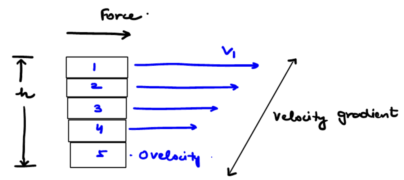
• $\dot{\gamma}$ — shear rate (velocity gradient), in reciprocal seconds ($\text{s}^{-1}$)
• $v$ — velocity of the topmost fluid layer, in metres per second ($\text{m/s}$)
• $h$ — height of the fluid layer, in metres ($\text{m}$)

Viscosity#

Viscosity is the internal resistance of a fluid to continuous shear deformation, or to the rate of strain, under an applied shear stress.

Kinematic viscosity#

Kinematic viscosity is the ratio of a fluid's dynamic viscosity to its density.

$$\nu = \frac{\mu}{\rho}$$

• $\nu$ — kinematic viscosity (momentum diffusivity — viscous effect on the fluid, independent of its mass or force), in square metres per second ($\text{m}^2/\text{s}$)
• $\mu$ — dynamic viscosity, in pascal-seconds ($\text{Pa} \cdot \text{s}$)
• $\rho$ — density of the fluid, in kilograms per cubic metre ($\text{kg/m}^3$)

Dividing out density leaves a purely kinematic quantity — no mass or force — which is why the Reynolds number can equivalently be written $Re = vd/\nu$, using kinematic rather than dynamic viscosity.

Power law equation (Ostwald–de Waele model)#

For non-Newtonian fluids only.

$$\tau = K \dot{\gamma}^n$$

• $\tau$ — shear stress, in pascals ($\text{Pa}$)
• $K$ — consistency index (generalized viscosity), in $\text{Pa} \cdot \text{s}^n$ (or $\text{N} \cdot \text{s}^n / \text{m}^2$): $K \uparrow \rightarrow$ viscosity $\uparrow$; $K \downarrow \rightarrow$ viscosity $\downarrow$
• $\dot{\gamma}$ — shear rate, in reciprocal seconds ($\text{s}^{-1}$)
• $n$ — flow behaviour index (exponent that classifies shear-thinning vs. shear-thickening behaviour), dimensionless

$n$	Fluid type	Behaviour
$n = 1$	Newtonian	—
$n > 1$	Dilatant (shear-thickening)	$\tau \uparrow \rightarrow \mu \uparrow$
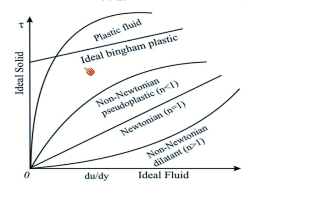
$n < 1$	Pseudoplastic (shear-thinning)	$\tau \uparrow \rightarrow \mu \downarrow$ — e.g. ketchup, which needs to be shaken

Apparent viscosity of a power-law fluid#

A non-Newtonian fluid has no single constant viscosity — it changes with shear rate. Restating the power law as an apparent viscosity ($\mu_a = \tau / \dot\gamma$) puts a shear-rate-dependent number in the same slot a constant $\mu$ would occupy, so it can be substituted directly into equations built for Newtonian fluids (e.g. the Reynolds number) at whatever shear rate the flow is actually running at.

$$\mu_a = K \dot{\gamma}^{\,n-1}$$

• $\mu_a$ — apparent viscosity (the effective, shear-rate-dependent viscosity of a non-Newtonian fluid at an instant — stands in for constant $\mu$ in equations built for Newtonian fluids), in pascal-seconds ($\text{Pa} \cdot \text{s}$)
• $K$ — consistency index, in $\text{Pa} \cdot \text{s}^n$
• $\dot{\gamma}$ — shear rate, in reciprocal seconds ($\text{s}^{-1}$)
• $n$ — flow behaviour index (exponent that classifies shear-thinning vs. shear-thickening behaviour), dimensionless

Worked example: apparent viscosity change with shear rate#

Question. For a power law fluid with flow behaviour index $n = 0.6$, if the shear rate is increased by a factor of $32$, by what factor does the apparent viscosity change?

Solution.

1. Start from $\mu_a = K \dot{\gamma}^{\,n-1}$.
2. $K$ is fixed for a given fluid, so it cancels in a ratio: $\dfrac{\mu_{a2}}{\mu_{a1}} = \left(\dfrac{\dot\gamma_2}{\dot\gamma_1}\right)^{n-1}$.
3. Substitute $\dot\gamma_2/\dot\gamma_1 = 32$ and $n - 1 = 0.6 - 1 = -0.4$.
4. $32^{-0.4} = (2^5)^{-0.4} = 2^{-2} = \dfrac{1}{4}$.
5. Sanity check: $n < 1$ is pseudoplastic (shear-thinning), so apparent viscosity must fall as shear rate rises — a ratio below $1$ is consistent.

Answer: Apparent viscosity decreases by a factor of $4$.

Worked example: reading $n$ off a log-log plot#

Question. In a log-log plot of shear stress ($\tau$) versus shear rate ($\dot{\gamma}$), the slope of the line equals $n$, the flow behaviour index. For a shear-thinning (pseudoplastic) fluid, what is the value of $n$?

Solution.

1. Start from the power law equation: $\tau = K \dot{\gamma}^n$.
2. Take the log of both sides: $\log \tau = \log K + n \log \dot{\gamma}$.
3. This is a straight line in $\log \tau$ vs. $\log \dot{\gamma}$ space, with slope $n$ and $y$-intercept $\log K$ — so the slope read off a log-log plot of $\tau$ against $\dot{\gamma}$ is exactly $n$.
4. A shear-thinning (pseudoplastic) fluid is defined, per the table above, by $n < 1$: apparent viscosity falls as shear stress rises.

Answer: $n < 1$ — the log-log line is shallower than the $n = 1$ Newtonian line (still positive slope, just less steep).

Newton's law of viscosity#

When $n = 1$, $K$ is replaced by $\mu$ (mu), the dynamic viscosity:

$$\tau = \mu \dot{\gamma} \quad \text{or} \quad \frac{\tau}{\dot{\gamma}} = \mu$$

• $\tau$ — shear stress, in pascals ($\text{Pa}$)
• $\mu$ — dynamic viscosity (constant for a Newtonian fluid — independent of the shear stress or shear rate applied), in pascal-seconds ($\text{Pa} \cdot \text{s}$)
• $\dot{\gamma}$ — shear rate, in reciprocal seconds ($\text{s}^{-1}$)

This is Newton's law of viscosity. Fluids that follow it are Newtonian fluids; fluids that don't are non-Newtonian fluids. Physical significance: for a Newtonian fluid, viscosity is constant — it is not affected by shear stress.

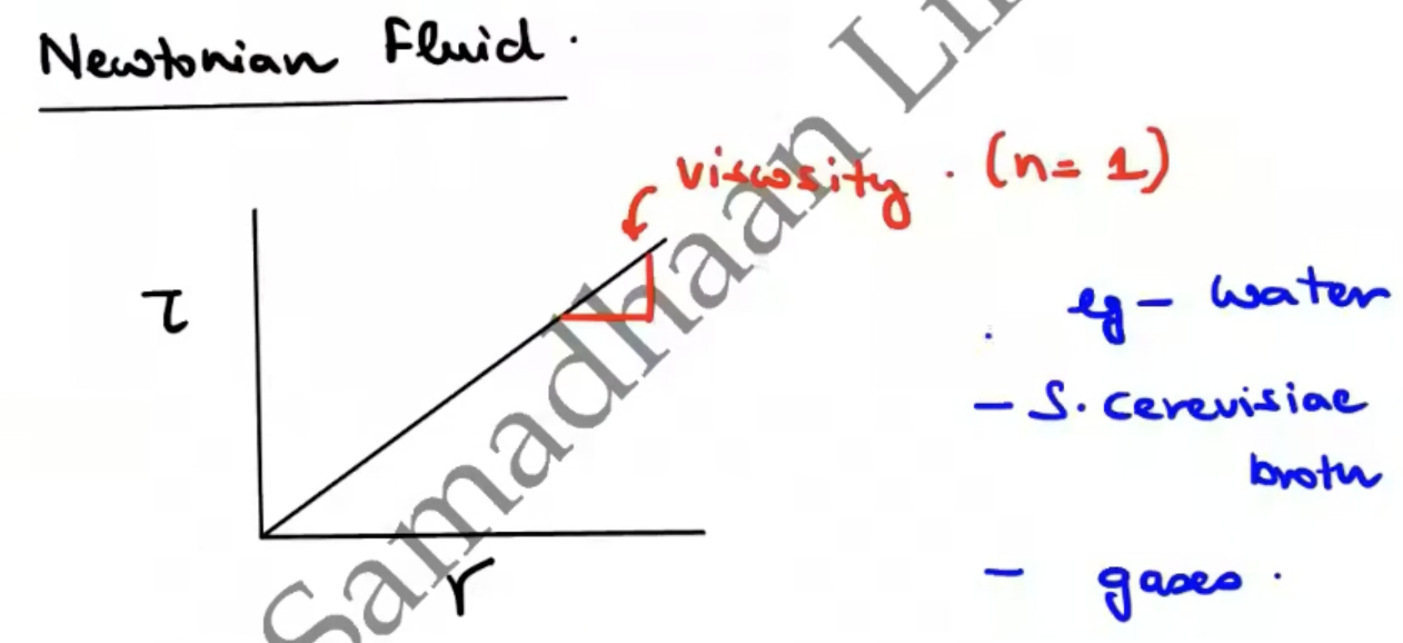
Examples of Newtonian fluids: water, Saccharomyces cerevisiae (S. cerevisiae) fermentation broth, and most gases.

Saccharomyces cerevisiae exhibits Newtonian behaviour at low biomass concentration; at high cell density (greater than 50 g/L dry cell weight), it becomes pseudoplastic — a fluid with dual nature.

Types of non-Newtonian fluids#

Bingham plastics#

A Bingham plastic is a solid below the yield stress, and a viscous Newtonian fluid above the yield stress.

Bingham plastics require a threshold shear stress — $\tau_0$ or $\tau_y$ (yield stress) — before any shear rate is generated at all.

$$\tau = \tau_y + \mu_p \dot{\gamma}$$

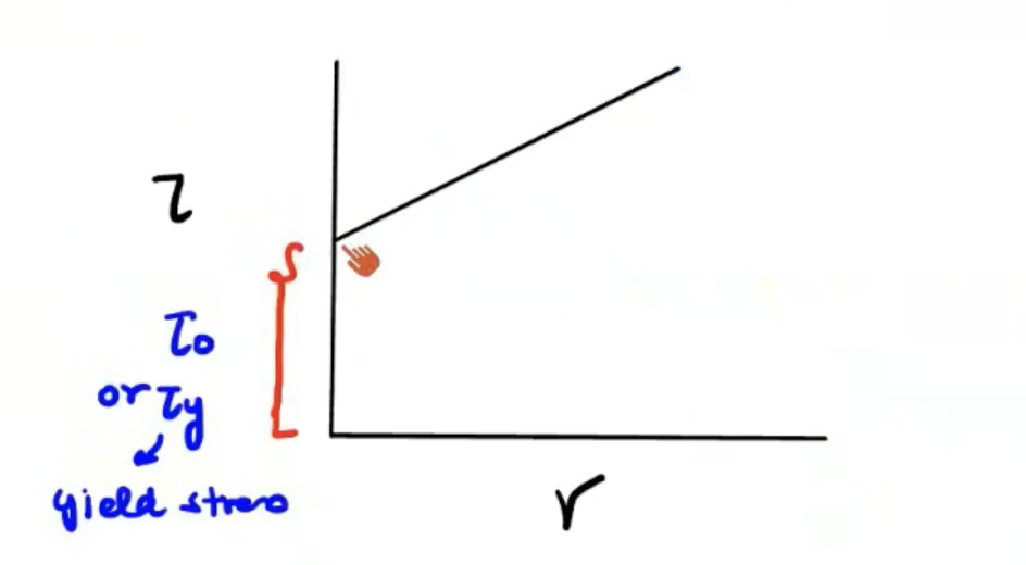
• $\tau$ — shear stress, in pascals ($\text{Pa}$)
• $\tau_y$ — yield stress (threshold stress that must be exceeded before the material begins to flow at all), in pascals ($\text{Pa}$)
• $\mu_p$ — plastic viscosity (also called apparent viscosity), in pascal-seconds ($\text{Pa} \cdot \text{s}$)
• $\dot{\gamma}$ — shear rate, in reciprocal seconds ($\text{s}^{-1}$)

Examples: tomato ketchup.

Pseudoplastics#

$n < 1$. As shear stress increases, apparent viscosity decreases: $\tau \uparrow \rightarrow \mu_a \downarrow$.

Examples: adhesives (e.g. Fevicol), polymer solutions, rubber solutions, xanthan gum, detergent slurry, mycelial fermentation broth, and human blood.

Dilatant#

$n > 1$. As shear stress increases, viscosity also increases: $\tau \uparrow \rightarrow \mu_a \uparrow$.

Examples: corn starch, cement slurry.

Casson plastics#

Casson fluids show dual nature:

• Below the threshold (yield) stress $\tau_0$: as $\tau$ increases, the fluid behaves like a Bingham plastic.
• Above $\tau_0$: as $\tau$ increases further, apparent viscosity decreases — $\tau \uparrow \rightarrow \mu_a \downarrow$.

$$\sqrt{\tau} = \sqrt{\tau_0} + \sqrt{K_c \dot{\gamma}}$$

• $\tau$ — shear stress, in pascals ($\text{Pa}$)
• $\tau_0$ — Casson yield stress (threshold stress below which the fluid behaves like a Bingham plastic), in pascals ($\text{Pa}$)
• $K_c$ — Casson viscosity coefficient, in pascal-seconds ($\text{Pa} \cdot \text{s}$)
• $\dot{\gamma}$ — shear rate, in reciprocal seconds ($\text{s}^{-1}$)

Examples: printing ink, tomato ketchup, orange juice, human blood, chocolate.

Human blood's yield stress comes from rouleaux formation: at low shear rates, red blood cells stack together like a column of coins, and breaking that stacked structure apart requires a threshold stress — the physical origin of blood's Casson-type yield behaviour. At higher shear rates the rouleaux break up and blood thins like a normal pseudoplastic fluid.

Herschel–Bulkley model#

The Herschel–Bulkley model generalizes Bingham plastics and power law fluids into one equation: a yield stress plus a power law response above it.

$$\tau = \tau_y + K \dot{\gamma}^n$$

• $\tau$ — shear stress, in pascals ($\text{Pa}$)
• $\tau_y$ — yield stress (threshold stress that must be exceeded before the material begins to flow at all), in pascals ($\text{Pa}$)
• $K$ — consistency index, in $\text{Pa} \cdot \text{s}^n$
• $\dot{\gamma}$ — shear rate, in reciprocal seconds ($\text{s}^{-1}$)
• $n$ — flow behaviour index (exponent that classifies shear-thinning vs. shear-thickening behaviour), dimensionless

Setting $\tau_y = 0$ recovers the power law equation; setting $n = 1$ recovers the Bingham plastic equation.

Comparing the fluid types#

Fluid type	$n$	Yield stress	Relation	Examples
Newtonian	$n = 1$	No	$\tau = \mu \dot{\gamma}$	Water, S. cerevisiae broth, most gases
Bingham plastic	—	Yes ($\tau_y$)	$\tau = \tau_y + \mu_p \dot{\gamma}$	Tomato ketchup
Pseudoplastic	$n < 1$	No	$\tau \uparrow \rightarrow \mu_a \downarrow$	Adhesives (Fevicol), polymer solutions, rubber solutions, xanthan gum, detergent slurry, mycelial fermentation broth, human blood
Dilatant	$n > 1$	No	$\tau \uparrow \rightarrow \mu_a \uparrow$	Corn starch, cement slurry
Casson plastic	—	Yes ($\tau_0$), dual nature	Bingham-like below $\tau_0$; pseudoplastic-like above	Printing ink, tomato ketchup, orange juice, human blood, chocolate

Time-dependent vs. time-independent non-Newtonian fluids#

Non-Newtonian fluids also split into two families based on whether apparent viscosity depends on the duration of shearing, not just its rate.

• Time-independent fluids: apparent viscosity depends only on the instantaneous shear rate or shear stress. Every type covered above — Bingham plastic, pseudoplastic, dilatant, Casson plastic, Herschel–Bulkley — is time-independent.
• Time-dependent fluids: apparent viscosity changes with how long a constant shear rate has been applied. Thixotropic and rheopectic fluids are the two types.

Thixotropic fluids#

A thixotropic fluid's apparent viscosity decreases over time under a constant shear rate, then recovers (thickens back up) once shearing stops and the fluid rests.

Examples: ketchup, yogurt, gels, paints, printer ink.

Rheopectic fluids#

A rheopectic (anti-thixotropic) fluid's apparent viscosity increases over time under a constant shear rate — the opposite of thixotropic behaviour. Rheopexy is rare.

Examples: gypsum paste, some clay suspensions, cream.

Comparing time-dependent fluids#

Fluid type	Apparent viscosity at constant shear rate	Examples
Thixotropic	Decreases with time	Ketchup, yogurt, gels, paints, printer ink
Rheopectic	Increases with time	Gypsum paste, some clay suspensions, cream

Worked example: time-dependent vs. time-independent classification (GATE-style)#

Question. Select the CORRECT statements regarding time-dependent and time-independent non-Newtonian fluids:

(A) Pseudoplastic fluids exhibit shear-thinning behaviour independent of the duration of shear. (B) Thixotropic fluids show a time-dependent decrease in apparent viscosity at a constant shear rate. (C) Rheopectic fluids show a time-dependent decrease in viscosity under constant shear. (D) Bingham plastics do not flow until the applied shear stress exceeds the threshold yield stress.

Solution.

1. Pseudoplastic fluids are time-independent: shear-thinning ($\mu_a \downarrow$ as $\dot\gamma \uparrow$) depends only on the instantaneous shear rate, not on how long shear has been applied — (A) is correct.
2. Thixotropic fluids are defined by exactly this: apparent viscosity falls over time at a fixed shear rate — (B) is correct.
3. Rheopectic fluids are the opposite of thixotropic: apparent viscosity increases over time at a fixed shear rate, not decreases — (C) is incorrect (it describes thixotropic behaviour, mislabeled as rheopectic).
4. Bingham plastics stay solid until $\tau$ exceeds the yield stress $\tau_y$, then flow like a Newtonian fluid — (D) is correct, matching $\tau = \tau_y + \mu_p \dot\gamma$.

Answer: A, B, and D are correct; C is incorrect.

Types of fluid flow#

Flow is classified into two regimes based on the pattern of fluid motion: laminar and turbulent.

Laminar flow (streamlined flow) moves in parallel layers, with streamlines that never cross. It is slow-moving and not recommended for mixing.

Turbulent flow is chaotic, irregular motion in which eddies form. It is recommended for mixing.

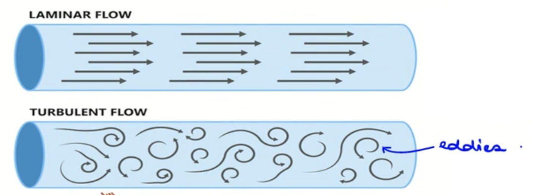
	Laminar flow	Turbulent flow
Pattern of motion	Parallel layers; streamlines do not cross	Chaotic, irregular
Velocity at a point	Steady with respect to time (non-chaotic)	Magnitude and direction both change; large, abrupt changes
Eddies	None	Formed
Speed	Slow-moving	—
Mixing	Not recommended	Recommended
Velocity profile across pipe diameter	Parabolic — maximum at the centreline, zero at the wall	Flatter (plug-like) across most of the diameter, dropping sharply only in a thin layer near the wall

Velocity profile in pipe flow#

In laminar pipe flow, momentum only transfers between adjacent layers by molecular viscosity, which produces a smooth parabolic velocity profile: fastest at the centreline, zero at the wall.

In turbulent pipe flow, the chaotic mixing from eddies constantly transfers momentum across the cross-section, dragging the near-wall fluid up and the centre fluid down — flattening the profile into a near-plug flow shape over most of the diameter, with a thin, steep drop confined to the wall region.

[Image to come — cross-section of a pipe comparing velocity profiles: laminar flow's smooth parabolic curve peaking at the centreline vs. turbulent flow's flatter, plug-like profile with a steep drop only near the wall]

Common confusion: vortex vs. turbulent flow#

Continuous rotation in a liquid produces a vortex. A vortex is often mistaken for turbulent flow, but it is not turbulent — it does not help mixing. Instead, it allows solids to settle out and precipitate toward the bottom.

Reynolds number#

The Reynolds number is the parameter that indicates whether a fluid is in laminar or turbulent flow. It represents the ratio of inertial forces to viscous forces in the fluid, and is dimensionless (unitless).

Reynolds number for stirred tank#

$$Re = \frac{d_i^2 N_i \rho}{\mu}$$

• $Re$ — Reynolds number (ratio of inertial to viscous forces), dimensionless
• $d_i$ — diameter of the impeller, in metres ($\text{m}$)
• $N_i$ — frequency of the impeller, in reciprocal seconds ($\text{s}^{-1}$)
• $\rho$ — density of the fluid, in kilograms per cubic metre ($\text{kg/m}^3$)
• $\mu$ — viscosity, in pascal-seconds ($\text{Pa} \cdot \text{s}$)
• $Re < 10$ — laminar
• $10 \le Re \le 10{,}000$ — transitional
• $Re > 10{,}000$ — turbulent

Reynolds number for straight pipe#

$$Re = \frac{d v \rho}{\mu}$$

• $Re$ — Reynolds number (ratio of inertial to viscous forces), dimensionless
• $d$ — diameter of the pipe, in metres ($\text{m}$)
• $v$ — average velocity of the fluid, in metres per second ($\text{m/s}$)
• $\rho$ — density of the fluid, in kilograms per cubic metre ($\text{kg/m}^3$)
• $\mu$ — viscosity, in pascal-seconds ($\text{Pa} \cdot \text{s}$)
• $Re < 2{,}100$ — laminar
• $Re > 4{,}000$ — turbulent

Flow regime by Reynolds number#

System	Laminar	Transitional	Turbulent
Stirred tank	$Re < 10$	$10 \le Re \le 10{,}000$	$Re > 10{,}000$
Straight pipe	$Re < 2{,}100$	—	$Re > 4{,}000$

Converting impeller speed: RPM to reciprocal seconds#

Impeller speed is often given in RPM (revolutions per minute), but $N_i$ in the equations above is in reciprocal seconds. Convert by dividing by 60:

$$N_i \, [\text{s}^{-1}] = \frac{N_i \, [\text{RPM}]}{60}$$

Froude number#

The Froude number is the parameter that represents the ratio of inertial forces to gravitational (buoyancy) forces.

At high impeller speed, inertial forces dominate gravity enough to distort the liquid's free surface — pulling it into a vortex and drawing in air — so $Fr$ is tracked alongside $Re$ during scale-up to catch that surface effect.

Froude number for stirred tank#

$$Fr = \frac{N_i^2 d_i}{g}$$

• $Fr$ — Froude number (ratio of inertial to gravitational/buoyancy forces), dimensionless
• $N_i$ — frequency of the impeller, in reciprocal seconds ($\text{s}^{-1}$)
• $d_i$ — diameter of the impeller, in metres ($\text{m}$)
• $g$ — acceleration due to gravity, $9.8 \ \text{m/s}^2$

Worked example: rheology models across fluid mechanics topics (GATE-style)#

Question. Which of the following statements regarding fluid rheology models is/are TRUE?

(a) The Casson equation is given by $\sqrt{\tau} = \sqrt{\tau_y} + \sqrt{K_c \dot\gamma}$. (b) For human blood, rouleaux formation at low shear rates contributes to yield stress behaviour. (c) Dilatant fluids show an increase in apparent viscosity with decreasing shear rate. (d) In pipe flow, turbulent flow has a flatter velocity profile across the tube diameter compared to laminar flow.

Solution.

1. (a) matches the Casson equation exactly ($\sqrt\tau = \sqrt{\tau_0} + \sqrt{K_c\dot\gamma}$, with $\tau_y$ here used interchangeably with $\tau_0$ for the yield stress) — correct.
2. (b) is the physical mechanism behind blood's yield-stress behaviour: red blood cells stack into rouleaux at low shear rates, and disrupting that structure needs a threshold stress — correct.
3. (c) inverts the definition of dilatant behaviour: $n > 1$ means $\tau \uparrow \rightarrow \mu_a \uparrow$, i.e. viscosity rises with increasing shear rate, not decreasing — incorrect.
4. (d) matches the velocity-profile comparison above: turbulent eddies redistribute momentum across the cross-section, flattening the profile into a near-plug shape versus laminar flow's parabolic profile — correct.

Answer: (a), (b), and (d) are correct; (c) is incorrect.

Key points#

• Ideal fluids are inviscid and incompressible (a hypothetical simplification); real fluids are viscous — compressibility is a separate, independent property.
• Newton's law of viscosity ($\tau = \mu\dot\gamma$) only holds for Newtonian fluids, where $\mu$ is constant; non-Newtonian fluids need an apparent viscosity ($\mu_a = K\dot\gamma^{\,n-1}$) that varies with shear rate instead.
• Flow behaviour index $n$ classifies non-Newtonian fluids: $n < 1$ pseudoplastic (shear-thinning), $n > 1$ dilatant (shear-thickening).
• Bingham plastics need a yield stress $\tau_y$ before they flow at all; Casson and Herschel–Bulkley fluids combine a yield stress with shear-thinning/power-law behaviour above it.
• Non-Newtonian fluids also split by time-dependence: Bingham, pseudoplastic, dilatant, Casson, and Herschel–Bulkley are all time-independent (viscosity depends only on instantaneous shear rate); thixotropic fluids thin over time at constant shear rate, rheopectic fluids thicken over time at constant shear rate.
• Reynolds number thresholds differ by system: stirred tank is laminar below $Re = 10$ and turbulent above $Re = 10{,}000$; straight pipe is laminar below $Re = 2{,}100$ and turbulent above $Re = 4{,}000$ — don't cross-apply the two.
• Turbulent flow (with eddies) is needed for mixing; laminar flow is not, and neither is a vortex — a vortex is easy to mistake for turbulence but actually promotes settling, not mixing.
• Laminar pipe flow gives a parabolic velocity profile (peak at centreline, zero at wall); turbulent pipe flow flattens it into a near-plug flow shape, with the steep drop confined to a thin near-wall layer.
• Human blood's Casson-type yield stress comes from rouleaux formation — red blood cells stacking at low shear rates — not from a generic "blood is thick" explanation.